43 how to show data labels in excel
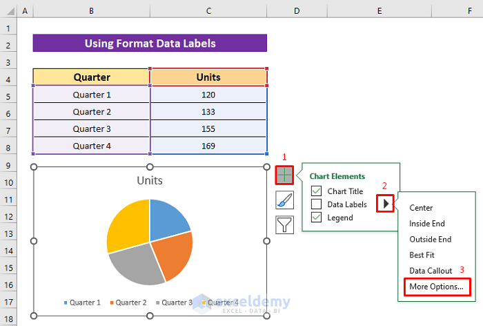
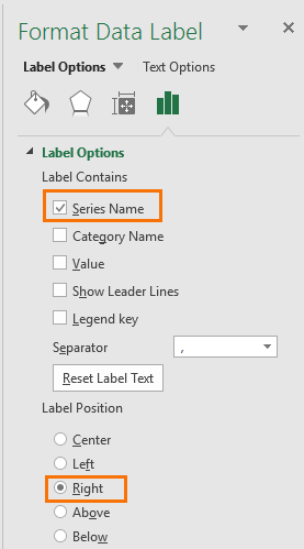
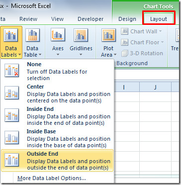
how to add data labels into Excel graphs - storytelling with data You can download the corresponding Excel file to follow along with these steps: Right-click on a point and choose Add Data Label. You can choose any point to add a label—I'm strategically choosing the endpoint because that's where a label would best align with my design. Excel defaults to labeling the numeric value, as shown below. How to Add Data Labels to an Excel 2010 Chart - dummies On the Chart Tools Layout tab, click Data Labels→More Data Label Options. The Format Data Labels dialog box appears. You can use the options on the Label Options, Number, Fill, Border Color, Border Styles, Shadow, Glow and Soft Edges, 3-D Format, and Alignment tabs to customize the appearance and position of the data labels.
Show or hide a chart legend or data table Show or hide a data table Click the chart of a line chart, area chart, column chart, or bar chart in which you want to show or hide a data table. This displays the Chart Tools , adding the Design , Layout , and Format tabs.

How to show data labels in excel
Format Data Labels in Excel- Instructions - TeachUcomp, Inc. To do this, click the "Format" tab within the "Chart Tools" contextual tab in the Ribbon. Then select the data labels to format from the "Chart Elements" drop-down in the "Current Selection" button group. Then click the "Format Selection" button that appears below the drop-down menu in the same area. Enable or Disable Excel Data Labels at the click of a button - How To Enable/Distable Data labels using form controls - Step by Step Step 1: Here is the sample data. Select and to go Insert tab > Charts group > Click column charts button > click 2D column chart. This will insert a new chart in the worksheet. Manage sensitivity labels in Office apps - Microsoft Purview ... Label display name of the label applied: General ${Item.Name} File name or email subject of the content being labeled: Sales.docx ${Item.Location} Path and file name of the document being labeled, or the email subject for an email being labeled \\Sales\2020\Q3\Report.docx ${User.Name} Display name of the user applying the label: Richard Simone
How to show data labels in excel. Custom Data Labels with Colors and Symbols in Excel Charts - [How To ... Step 4: Select the data in column C and hit Ctrl+1 to invoke format cell dialogue box. From left click custom and have your cursor in the type field and follow these steps: Press and Hold ALT key on the keyboard and on the Numpad hit 3 and 0 keys. Let go the ALT key and you will see that upward arrow is inserted. How to I rotate data labels on a column chart so that they are ... To change the text direction, first of all, please double click on the data label and make sure the data are selected (with a box surrounded like following image). Then on your right panel, the Format Data Labels panel should be opened. Go to Text Options > Text Box > Text direction > Rotate Custom Chart Data Labels In Excel With Formulas - How To Excel At Excel Follow the steps below to create the custom data labels. Select the chart label you want to change. In the formula-bar hit = (equals), select the cell reference containing your chart label's data. In this case, the first label is in cell E2. Finally, repeat for all your chart laebls. Excel tutorial: How to use data labels Generally, the easiest way to show data labels to use the chart elements menu. When you check the box, you'll see data labels appear in the chart. If you have more than one data series, you can select a series first, then turn on data labels for that series only. You can even select a single bar, and show just one data label.
How to add data labels from different column in an Excel chart? Click any data label to select all data labels, and then click the specified data label to select it only in the chart. 3. Go to the formula bar, type =, select the corresponding cell in the different column, and press the Enter key. See screenshot: 4. Repeat the above 2 - 3 steps to add data labels from the different column for other data points. How to Add Axis Labels in Excel Charts - Step-by-Step (2022) - Spreadsheeto How to add axis titles 1. Left-click the Excel chart. 2. Click the plus button in the upper right corner of the chart. 3. Click Axis Titles to put a checkmark in the axis title checkbox. This will display axis titles. 4. Click the added axis title text box to write your axis label. How to Add Labels to Show Totals in Stacked Column Charts in Excel Press the Ok button to close the Change Chart Type dialog box. The chart should look like this: 8. In the chart, right-click the "Total" series and then, on the shortcut menu, select Add Data Labels. 9. Next, select the labels and then, in the Format Data Labels pane, under Label Options, set the Label Position to Above. 10. How to show percentage in pie chart in Excel? - ExtendOffice Show percentage in pie chart in Excel. Please do as follows to create a pie chart and show percentage in the pie slices. 1. Select the data you will create a pie chart based on, click Insert > Insert Pie or Doughnut Chart > Pie. See screenshot: 2. Then a pie chart is created. Right click the pie chart and select Add Data Labels from the context ...
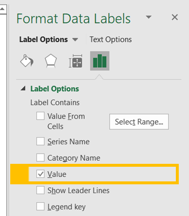
Add a DATA LABEL to ONE POINT on a chart in Excel Click on the chart line to add the data point to. All the data points will be highlighted. Click again on the single point that you want to add a data label to. Right-click and select ' Add data label ' This is the key step! Right-click again on the data point itself (not the label) and select ' Format data label '. Excel, giving data labels to only the top/bottom X% values 1) Create a data set next to your original series column with only the values you want labels for (again, this can be formula driven to only select the top / bottom n values). See column D below. 2) Add this data series to the chart and show the data labels. 3) Set the line color to No Line, so that it does not appear! Excel charts: how to move data labels to legend @Matt_Fischer-Daly . You can't do that, but you can show a data table below the chart instead of data labels: Click anywhere on the chart. On the Design tab of the ribbon (under Chart Tools), in the Chart Layouts group, click Add Chart Element > Data Table > With Legend Keys (or No Legend Keys if you prefer) How to create Custom Data Labels in Excel Charts - Efficiency 365 Two ways to do it. Click on the Plus sign next to the chart and choose the Data Labels option. We do NOT want the data to be shown. To customize it, click on the arrow next to Data Labels and choose More Options … Unselect the Value option and select the Value from Cells option. Choose the third column (without the heading) as the range.
Show Trend Arrows in Excel Chart Data Labels
How to Make a Pie Chart in Excel & Add Rich Data Labels to 08.09.2022 · A pie chart is used to showcase parts of a whole or the proportions of a whole. There should be about five pieces in a pie chart if there are too many slices, then it’s best to use another type of chart or a pie of pie chart in order to showcase the data better. In this article, we are going to see a detailed description of how to make a pie chart in excel.

Add or remove data labels in a chart
Change the format of data labels in a chart To get there, after adding your data labels, select the data label to format, and then click Chart Elements > Data Labels > More Options. To go to the appropriate area, click one of the four icons ( Fill & Line, Effects, Size & Properties ( Layout & Properties in Outlook or Word), or Label Options) shown here.

Change the format of data labels in a chart
How to Use Cell Values for Excel Chart Labels - How-To Geek Mar 12, 2020 · Make your chart labels in Microsoft Excel dynamic by linking them to cell values. When the data changes, the chart labels automatically update. In this article, we explore how to make both your chart title and the chart data labels dynamic. We have the sample data below with product sales and the difference in last month’s sales.

Google Workspace Updates: Get more control over chart data ...
Add or remove data labels in a chart - support.microsoft.com Data labels make a chart easier to understand because they show details about a data series or its individual data points. For example, in the pie chart below, without the data labels it would be difficult to tell that coffee was 38% of total sales. Depending on what you want to highlight on a chart, you can add labels to one series, all the ...

Adding rich data labels to charts in Excel 2013 | Microsoft ...
How to show data label in "percentage" instead of - Microsoft Community Select Format Data Labels Select Number in the left column Select Percentage in the popup options In the Format code field set the number of decimal places required and click Add. (Or if the table data in in percentage format then you can select Link to source.) Click OK Regards, OssieMac Report abuse 8 people found this reply helpful ·

charts - Excel, giving data labels to only the top/bottom X ...
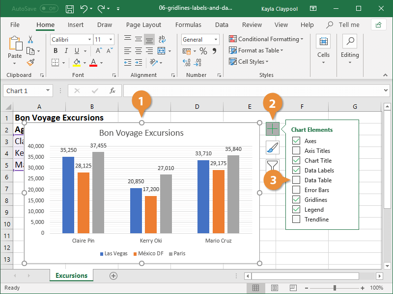
How to add or move data labels in Excel chart? - ExtendOffice 1. Click the chart to show the Chart Elements button . 2. Then click the Chart Elements, and check Data Labels, then you can click the arrow to choose an option about the data labels in the sub menu. See screenshot:

microsoft excel - Adding data label only to the last value ...
How to Rename a Data Series in Microsoft Excel - How-To Geek 27.07.2020 · A data series in Microsoft Excel is a set of data, shown in a row or a column, which is presented using a graph or chart. To help analyze your data, you might prefer to rename your data series. Rather than renaming the individual column or row labels, you can rename a data series in Excel by editing the graph or chart. You might want to do this ...

Apply Custom Data Labels to Charted Points - Peltier Tech
Fix Excel Pivot Table Missing Data Field Settings - Contextures Excel … Aug 31, 2022 · Show Missing Data. To show missing data, such as new products, you can add one or more dummy records to the pivot table, to force the items to appear. For example, to include a new product -- Paper -- in the pivot table, even if it has not yet been sold: In the source data, add a record with Paper as the product, and 0 as the quantity; Refresh ...

Apply Custom Data Labels to Charted Points - Peltier Tech
How to show values in data labels of Excel Pareto Chart when chart is ... They wish to show data labels above each column to indicate the number of occurrences. So for example, they may have 6 events on the x-axis: ... for category labels, the second for the bars (percentages), and the third for the line cumulative percentages). I added data labels to the bars, using Excel 2013's option to use label text from cells ...

How to Make Pie Chart with Labels both Inside and Outside ...
How to identify duplicates in Excel: find, highlight, count, filter To display all duplicate records, i.e. occurrences greater than 1, click the filter arrow in the header of the Occurrences column (the column with the formula), and then click Number Filters > Greater Than. Select " is greater than " in the first box, type 1 in the box next to it, and click the OK button:
/Capture-e92aa05671d543ceaf94080eb2687619.JPG)
Understanding Excel Chart Data Series, Data Points, and Data ...
Find, label and highlight a certain data point in Excel scatter graph Select the Data Labels box and choose where to position the label. By default, Excel shows one numeric value for the label, y value in our case. To display both x and y values, right-click the label, click Format Data Labels…, select the X Value and Y value boxes, and set the Separator of your choosing: Label the data point by name

How can I hide 0% value in data labels in an Excel Bar Chart ...
Excel data doesn't retain formatting in mail merge - Office 31.03.2022 · In the Select Data Source dialog box, locate the folder that contains the Excel workbook that you want to use as your data source, select workbook, and then select Open. In the Confirm Data Source dialog box, select to select the Show all check box. select MS Excel Worksheets via DDE (*.xls) , and then select OK .

Add or remove data labels in a chart
How to Show Percentage in Pie Chart in Excel? - GeeksforGeeks 29.06.2021 · It can be observed that the pie chart contains the value in the labels but our aim is to show the data labels in terms of percentage. Show percentage in a pie chart: The steps are as follows : Select the pie chart. Right-click on it. A pop-down menu will appear. Click on the Format Data Labels option. The Format Data Labels dialog box will appear.

how to add data labels into Excel graphs — storytelling with data
How to Add Labels to Scatterplot Points in Excel - Statology Step 3: Add Labels to Points. Next, click anywhere on the chart until a green plus (+) sign appears in the top right corner. Then click Data Labels, then click More Options…. In the Format Data Labels window that appears on the right of the screen, uncheck the box next to Y Value and check the box next to Value From Cells.

Improve your X Y Scatter Chart with custom data labels
Directly Labeling in Excel - Evergreen Data There are two ways to do this. Way #1. Click on one line and you'll see how every data point shows up. If we add a label to every data points, our readers are going to mount a recall election. So carefully click again on just the last point on the right. Now right-click on that last point and select Add Data Label.

Microsoft Excel Tutorials: Add Data Labels to a Pie Chart
How to Change Excel Chart Data Labels to Custom Values? Now, click on any data label. This will select "all" data labels. Now click once again. At this point excel will select only one data label. Go to Formula bar, press = and point to the cell where the data label for that chart data point is defined. Repeat the process for all other data labels, one after another. See the screencast. Points to note:

microsoft excel - Adding data label only to the last value ...
How To Add Data Labels In Excel - politicast.info To get there, after adding your data labels, select the data label to format, and then click chart elements > data labels > more options. After picking the series, click the data point you want to label. Source: temotips.blogspot.com. Using excel chart element button to add axis labels. Click the chart to show the chart elements button.

Custom data labels in a chart
How to Add Total Data Labels to the Excel Stacked Bar Chart 03.04.2013 · For stacked bar charts, Excel 2010 allows you to add data labels only to the individual components of the stacked bar chart. The basic chart function does not allow you to add a total data label that accounts for the sum of the individual components. Fortunately, creating these labels manually is a fairly simply process.
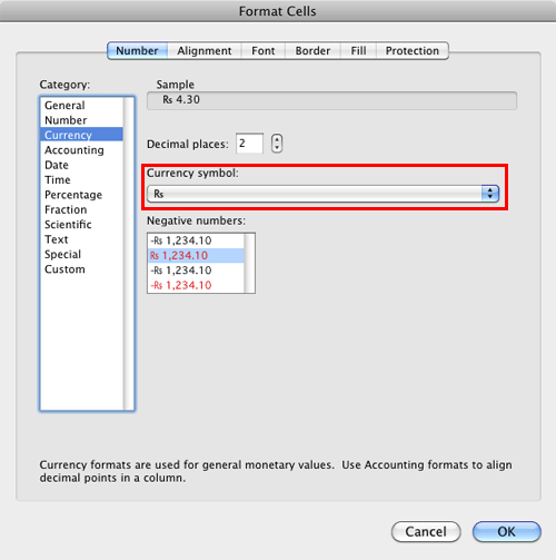
Format Number Options for Chart Data Labels in Excel 2011 for Mac
Manage sensitivity labels in Office apps - Microsoft Purview ... Label display name of the label applied: General ${Item.Name} File name or email subject of the content being labeled: Sales.docx ${Item.Location} Path and file name of the document being labeled, or the email subject for an email being labeled \\Sales\2020\Q3\Report.docx ${User.Name} Display name of the user applying the label: Richard Simone

Total of chart series – Excel kitchenette
Enable or Disable Excel Data Labels at the click of a button - How To Enable/Distable Data labels using form controls - Step by Step Step 1: Here is the sample data. Select and to go Insert tab > Charts group > Click column charts button > click 2D column chart. This will insert a new chart in the worksheet.

Apply Custom Data Labels to Charted Points - Peltier Tech
Format Data Labels in Excel- Instructions - TeachUcomp, Inc. To do this, click the "Format" tab within the "Chart Tools" contextual tab in the Ribbon. Then select the data labels to format from the "Chart Elements" drop-down in the "Current Selection" button group. Then click the "Format Selection" button that appears below the drop-down menu in the same area.

How to show data labels in PowerPoint and place them ...

How to Add Two Data Labels in Excel Chart (with Easy Steps ...

Adding rich data labels to charts in Excel 2013 | Microsoft ...

Add or remove data labels in a chart

How to Change Excel Chart Data Labels to Custom Values?

How to add or move data labels in Excel chart?
How to Show Pie Chart Data Labels in Percentage in Excel
Solved: Area chart data labels not in correct positions ...

Change the format of data labels in a chart

Chart axes, legend, data labels, trendline in Excel - Tech Funda

Is there a way to show different data labels in a bar chart ...
How to Add Axis Labels to a Chart in Excel | CustomGuide
Dynamically Label Excel Chart Series Lines • My Online ...
How to Show Percentages in Stacked Column Chart in Excel ...

data visualization - How do you put values over a simple bar ...

How to Use Cell Values for Excel Chart Labels

Change the format of data labels in a chart

perl - Excel::Writer::XLSX - Data Label "Value From Cells ...
Excel 2010: Show Data Labels In Chart

How-to Use Data Labels from a Range in an Excel Chart - Excel ...

Adding rich data labels to charts in Excel 2013 | Microsoft ...
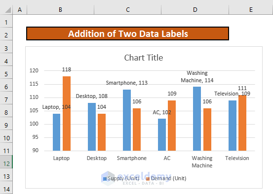
How to Add Two Data Labels in Excel Chart (with Easy Steps ...
Post a Comment for "43 how to show data labels in excel"